D&C Schedule Builder
D&C Schedule Builder — User Manual
1. What Is the D&C Schedule Builder?
The D&C Schedule Builder is a field development planning tool that lets you build, visualize, and optimize a drilling and completion (D&C) schedule across multiple pads. It automatically forecasts production based on a configurable type-well curve, enforces rig capacity constraints, and optionally models Parent-Child (PC) interference between adjacent wells.
The tool is organized around three main panels:
| Panel | Location | Purpose |
|---|---|---|
| D&C Settings | Left sidebar | Global drilling/completion parameters and forecast dates |
| Timeline View / Gantt Chart | Center (Tab 1) | Visual schedule with draggable bars per pad |
| Parent-Child Config | Center (Tab 2) | Configuration of interference math and degradation curves |
| Spatial View | Center (Tab 3) | Interactive 2D/3D development map with timeline animation |
| PAD SCHEDULE | Right | Table of all pads and wells with dates, spacing, and production metrics |
| Production Chart | Bottom | Field-wide production forecast (rates and cumulatives) |
2. Interface Overview
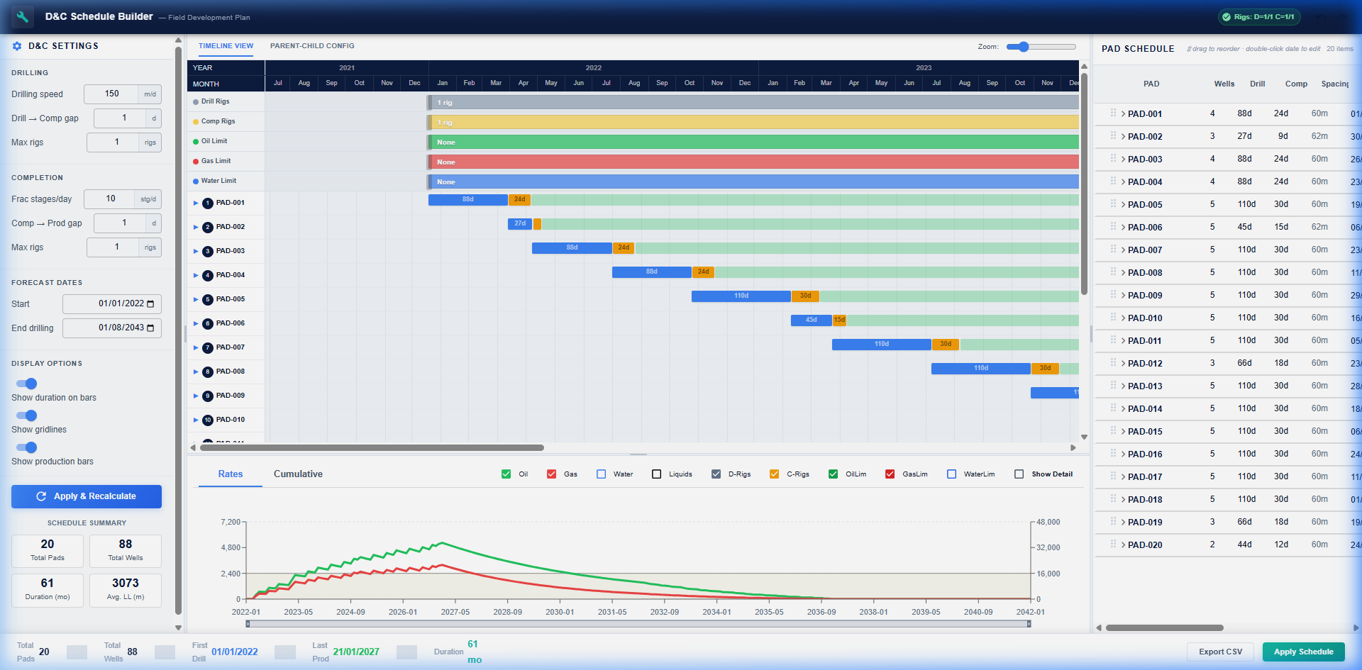
The main screen shows the Timeline View, which combines:
- The Gantt chart (center) — one row per pad, showing drilling bars, completion bars, and production onset
- The PAD SCHEDULE table (right) — editable pad metadata and per-well metrics
- The Production Chart (bottom) — total field production curves for oil, gas, water, and liquids
- The D&C Settings panel (left) — global rig counts, duration parameters, and date range
3. D&C Settings Panel
The left-hand settings panel controls the global schedule parameters that apply to all pads.
3.1 Drilling
| Setting | Description |
|---|---|
| Drilling Speed (m/d) | Lateral drilling rate in metres per day. Controls how long drilling takes per pad based on the average lateral length. |
| Drill → Comp Gap (days) | Waiting time between end of drilling and start of completion (frac) operations. |
| Max Rigs | Maximum simultaneous drilling rigs active at any time. |
3.2 Completion
| Setting | Description |
|---|---|
| Frac Stages/day | Completion pace, in frac stages per day. Controls how long the frac job takes per well based on lateral length and spacing. |
| Comp → Prod Gap (days) | Waiting time between end of completion and first production (flowback period). |
| Max Rigs | Maximum simultaneous completion (frac) crews. |
3.3 Forecast Dates
| Setting | Description |
|---|---|
| Start | The first date from which the forecasted production curves are shown. |
| End Drilling | The last date on which new drilling operations can begin. Pads scheduled beyond this date are excluded. |
3.4 Display Options
- Show duration on bars — Displays the number of days on each Gantt bar for quick reference.
- Show gridlines — Toggles vertical monthly gridlines on the Gantt chart.
- Show production bars — Toggles visibility of the production onset indicator on the Gantt.
3.5 Apply & Recalculate
After modifying any setting, press Apply & Recalculate to regenerate the schedule dates, enforce rig constraints, and update all production forecasts.
4. Gantt Chart (Timeline View)
The Gantt chart shows one row per pad with three types of bars:
| Bar Type | Color | Meaning |
|---|---|---|
| Drilling | Grey/dark | Period during which the rig is drilling the pad’s laterals |
| Completion | Yellow/amber | Period during which the completion crew is fracturing the wells |
| Production | (thin line or dot) | First production date for the pad |
| PC Interference marker | Red dot | Indicates that at least one well in this pad is affected by a Parent well |
4.1 Reordering Pads
Pads can be dragged vertically to reorder them. The scheduler will automatically reassign dates based on the new order, subject to rig availability constraints.
4.2 Adjusting Rig Segments
The production limit and rig count bars at the top of the chart can be dragged horizontally to define time periods with different rig counts or rate limits. Double-click on a segment to edit its value directly.
5. PAD SCHEDULE Table
The right-hand panel shows a table of all pads in the schedule. Each row represents one pad, with key metrics displayed in standardized columns.
5.1 Pad-Level Columns
| Column | Description |
|---|---|
| PAD | Pad identifier |
| Wells | Number of wells in the pad |
| Drill (days) | Total drilling duration for the pad |
| Comp (days) | Total completion (frac) duration for the pad |
| Spacing (m) | Well spacing within the pad |
| Drill Start | First day of drilling operations |
| Drill End | Last day of drilling operations |
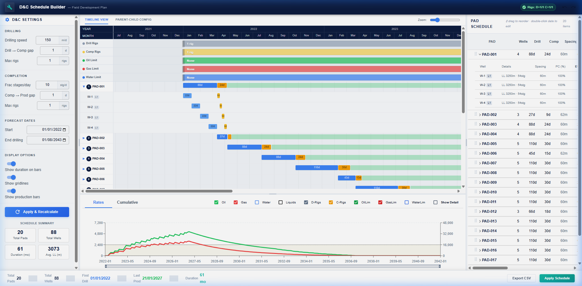
5.2 Expanding a Pad — Well-Level Metrics
Click the expand arrow (▶) next to any pad name to reveal the individual wells and their Parent-Child production metrics:
| Column | Description |
|---|---|
| Well | Well name and type-well profile |
| LL (m) | Lateral length of the well |
| Stages | Number of frac stages |
| Spacing (m) | Frac stage spacing |
| PC (%) | Productivity Factor from PC interference: 100% = no interference, e.g., 85% = 15% reduction |
| EUR Oil (Mm³) | Estimated Ultimate Recovery of oil in thousands of cubic metres, after PC degradation |
| EUR Gas (MMm³) | EUR gas in millions of cubic metres, after PC degradation |
| EUR BOE (MMBOE) | Combined EUR in Million Barrels of Oil Equivalent (using 5,615 scf/BOE) |
Note: If PC effects are disabled or the well is not within the interference radius of any parent, PC% = 100% and EUR values equal the full type-well forecast.
6. Production Chart
The bottom panel shows the full field-wide production forecast over the entire schedule horizon.
6.1 Tabs
| Tab | Description |
|---|---|
| Rates | Monthly average production rates in m³/d (oil/water/liquids) and Mm³/d (gas) |
| Cumulative | Cumulative produced volumes. Reconciliation Proof: Field-wide totals are mathematically re-derived as the exact sum of individual pad contributions at every month, ensuring 100% UI consistency. |
6.2 Toggle Checkboxes
The checkboxes at the top of the chart control which curves are visible:
| Toggle | Description |
|---|---|
| Oil / Gas / Water / Liquids | Show/hide each fluid type |
| D-Rigs / C-Rigs | Show/hide rig count areas as shaded background zones |
| OilLim / GasLim / WaterLim | Show/hide production rate constraint lines |
| Show Detail | Overlay individual per-pad production curves (dashed lines) on top of the total (solid lines) |
6.3 Zoom and Pan
The horizontal brush bar at the bottom of the chart can be dragged at either end to zoom into a specific date range. The chart axes will automatically rescale.
7. Parent-Child (PC) Interference Configuration
Navigate to the PARENT-CHILD CONFIG tab to configure interference effects.
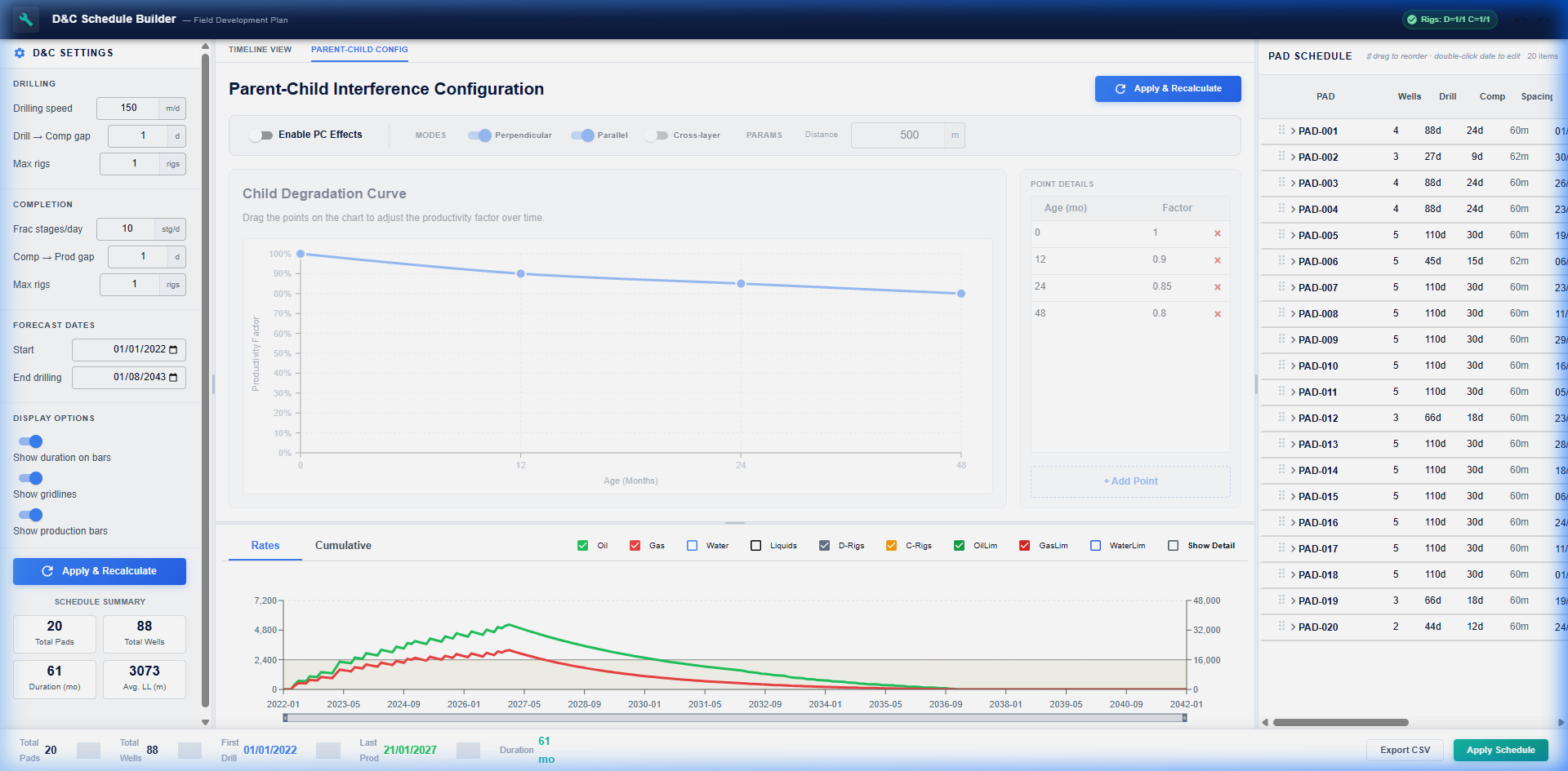
7.1 Enable PC Effects
The master toggle that activates or deactivates all Parent-Child calculations. When disabled, all wells show PC = 100% and EUR values equal the full type-well.
7.2 Interference Modes
The system uses a Head-Heel-Toe geometric model to precisely locate horizontal wells in space. Proximity is evaluated strictly between the lateral segments (Heel to Toe) to ensure interference is reservoir-driven.
Three spatial modes control how proximity is evaluated:
| Mode | Description |
|---|---|
| Perpendicular | Calculates the distance between the geometric midpoints of the two lateral segments. This is ideal for identifying primary side-by-side interference. |
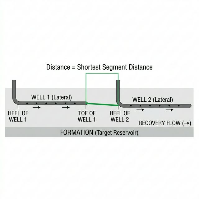
| Parallel | Calculates the shortest distance between any two points on the two laterals. This mode captures “Toe-to-Heel” adjacency for wells following each other or staggered patterns. |
| Cross-layer | If enabled, wells in different landing zones (formation benches) can interfere with each other. |
Educational Help: Click the ’?’ icon next to each mode to open a specialized, book-style diagram that illustrates the calculation logic with visual well-pad examples.

Multiple modes can be active simultaneously. When both Perpendicular and Parallel are enabled, the minimum distance found by either mode is used.
7.3 Interference Distance (m)
The maximum spatial distance (in metres) within which a child well is considered affected by a parent. Typical values range from 200 m to 600 m depending on the formation and fracture half-length. Wells beyond this threshold are unaffected regardless of timing.
7.4 Child Degradation Curve
This curve defines the productivity factor as a function of how long the parent has been producing before the child starts:
- X-axis (Age, months) — time elapsed between parent first production and child first production
- Y-axis (Productivity Factor) — fraction of the child’s full type-well performance (1.0 = no degradation, 0.0 = total loss)
Editing the curve:
- Drag any point on the curve to adjust the factor at that age
- Click + Add Point to insert a new control point
- Click the × button next to a row in the table to remove a point
- The curve is interpolated using a smooth monotone spline between control points
7.5 Applying Changes
After adjusting any PC parameters, click Apply & Recalculate to recompute well factors, update the PAD SCHEDULE metrics, and refresh the production chart.
8. Spatial Development View
The SPATIAL VIEW tab provides an interactive geographic visualization of your development plan. It is designed to verify well placement and monitor interference in real-time.
(Image: 3D Spatial Map showing active development - File omitted)
8.1 3D Navigation (WebGL)
In 3D mode, you can move freely through the reservoir:
- Rotate: Left-click and drag to orbit around the field.
- Zoom: Use the mouse wheel to move closer or further away.
- Pan: Right-click and drag to move the camera horizontally/vertically.
- Compass Gizmo: A 3D axis compass in the bottom right corner helps maintain spatial orientation.
- North Alignment: Use the
NORTHbutton in the toolbar to instantly snap the 3D camera to a top-down, North-aligned view.
8.1b 3D Well Geometry
- Cylindrical Segments: Well laterals are rendered as solid 3D cylinders with distinct white contour highlights (wireframe edges), providing a clear sense of volume and depth structure.
8.2 Synchronized Timeline Scrubber
The floating overlay at the bottom allows you to “playback” your schedule:
- Manual Scrubbing: Drag the handle to jump to any month in the schedule.
- Play/Pause: Automate the visual progress of drilling and production.
- Visual Feedback: Wells change color as they progress from ‘Drilling’ (Orange) to ‘Producing’ (Green/Red).
8.3 Well PC Factor Color Scale
To quickly identify low-performing areas, well laterals (Heel-to-Toe) are colored based on their Parent-Child productivity factor:
- Green (100%): No interference, full production.
- Gradient: Transitions through yellow and orange.
- Red (Low %): Significant interference from a parent well.
8.4 Minimalist Tags and Indicators
To maintain a clean interface, well names and interference halos are hidden by default. Use the TAGS button in the header to toggle them:
- OFF (Default): Clean map showing only paths and status.
- ON: Small white tags appear at the Toe of each well. Affected producing wells will display a pulsing red halo and their exact PC percentage (e.g., “PC 85%“).
8.5 2D Parity Mode
Switch to 2D in the header for a flat, top-down view. This mode supports the same timeline scrubbing, well selection, and tag toggles as the 3D mode, optimized for layout planning.
9. Typical Workflow
- Load optimizer data — The scheduler reads pad and well geometry from the optimizer response file automatically on startup.
- Review the default schedule — The Gantt chart shows the default pad order with dates derived from rig availability and D&C durations.
- Adjust D&C Settings — Tune drilling speed, rig counts, and gap times to match your operational assumptions.
- Reorder pads — Drag pads in the Gantt to change drilling priority and observe how dates shift.
- Enable PC Effects — Navigate to the Parent-Child Config tab, set the interference distance and degradation curve, and apply.
- Review well metrics — Expand pads in the PAD SCHEDULE table to check PC% and EUR values for each well.
- Analyze the production forecast — Use the Production Chart to compare field-wide rates and cumulatives with and without PC effects.
- Export — Use the Export CSV button in the PAD SCHEDULE table to export the schedule and metrics to a spreadsheet.