Type Well

The Type well feature allows users to calculate one or more type wells, using two different methods:

• From statistics: based on multiple forecasts, assuming a lognormal probability distribution.

• User defined: manual input parameters provided by the user.

The feature is located over ‘Analysis’ tab in the navbar, inside ‘Decline Curve Analysis’ section.

Decline Curve Analysis in the main toolbar

Type Well from Statistics

The Type Well from Statistics feature allows the user to calculate one or more type wells, fitting forecasted initial rates and EURs, assuming a lognormal probability distribution.

The feature will be located over ‘Analysis’ tab in the navbar, inside ‘Decline Curve Analysis’ section.

Type Well from statistics in the main toolbar

Initial rate tab parameters

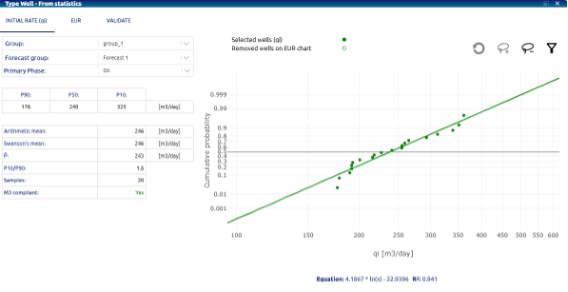Type Well – Initial rate tab

• Well group: dropdown for selecting the group of wells to choose the forecast

• Forecast group: dropdown for selecting the forecast for use in determining statistics

• Primary phase: dropdown for selecting well forecasts primary phase. Options:

    o Oil

    o Gas

• Percentiles P90, P50, P10: percentiles for the data set for the initial flow rate (qi) in the wells included in the analysis. Percentiles divide the data into 100 equal parts, with each representing the value below which a certain percentage of the data falls. In this way, P90 is the value below which 90% of the data is found. In our case, it represents a pessimistic scenario, with the most optimistic case being the value shown by P10.

• Custom Percentiles: Additionally, the user can now select a type well with a custom percentile, which will be incorporated into the calculation table.

• Arithmetic mean: It is the simple average of a set of values for qi, calculated as the sum of all the values divided by the number of values, represents the average value of the data.

• Swanson’s mean: Calculated as a weighted average using key percentiles, it provides a representative estimate that incorporates both the range (P90 and P10) and the center value (P50) of the data.

• P̂: Expected value is used to represent the expected average result of a random variable, taking into account uncertainty.

• P10/P90: It is the relationship between the 10th percentile and the 90th percentile, calculated as: P10/P90. Indicates the degree of dispersion or uncertainty in the data. A ratio close to 1 suggests that the distribution is narrow (less uncertainty), a very low ratio indicates high dispersion and greater uncertainty.

• Samples: number of qi values (number of wells) included in the analysis.

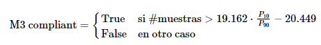
• M3 compliant: the model complies with the M3 standard, ensures that the mean, median, and mode of the distribution are in a logical or coherent relationship within the data set.

• Chart: is a visual representation of how the values of that variable are distributed in terms of cumulative probability. A curve with a steep slope would indicate that the initial flow values are concentrated in a narrow range, suggesting low dispersion, a flatter curve that the values are more dispersed, indicating greater variability or uncertainty.

• Chart toolbar: allows you to interact with the graph to select/deselect qi points to be included or not in the calculation, you can also access the list of wells used and perform this filter based on the well name.

EUR tab parameters

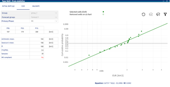Type Well – EUR tab

The same statistics applied to the variable that are used in this tab taking EUR (Estimated Ultimate Recovery) as the variable, in this case the Group and the Forecast group cannot be modified from the choice made in the first tab, being able to intervene on the choice of wells within the group to be considered in the analysis.

Validate tab parameters

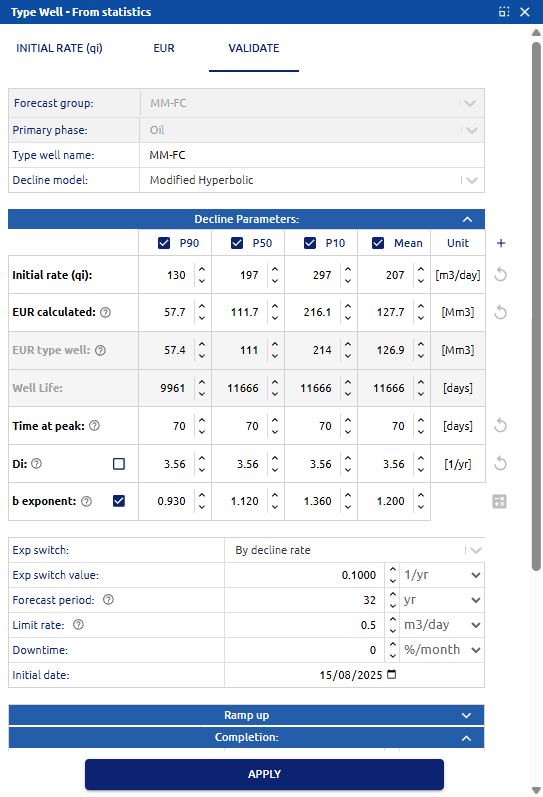Type Well – Validate tab

• Forecast group: shows the forecast selected in the initial tab to determine the statistics

• Primary phase: showos the well forecasts primary phase selected.

• Decline Model: dropdown for selecting type well forecasts decline model. Options:

    o Exponential (Exp)

    o Hyperbolic (H)

    o Modified hyperbolic (MH)

    o Power law exponential (PLE)

    o Stretched exponential (SE)

• Decline parameters: a decline is generated for each of the three percentiles (P10, P50 and P90) and the “Mean well” calculated with the Arithmetic mean, taking as input the values of initial rate (qi) and EUR determined in the previous steps. In addition to these two parameters, and depending on the decline model chosen, the following are also included (initially estimated as the average of the individual values for the wells included in the analysis.):

    o Time at peak: time at peak rate, expressed in days.

    o (only for H / MH / Exp decline models) Di: initial decline rate, expressed
      in 1/yr.

    o (only for H / MH decline models) b exponent: parameter that characterizes
      the form of declination of hyperbolic curves.

    o (only for PLE / SE decline models) n exponent: power-law exponent, describes
      how the rate of decline changes over time.

    o (only for PLE / SE decline models) transition time: tau factor, expressed
      in days. Factor that is related to the characteristic time of decline and
      modulates how the production rate declines over time.

    o (only for MH decline models) Exp Switch: indicates the condition for switching
      from Hyperbolic to Exponential function. Options: by time (time), by decline
      rate (1/time)

    o (only for MH decline models) Exp Switch value: value to enter according
      to the chosen switch option

    o Forecast period: Indicates the number of years up to which to forecast.

    o Limit rate: Indicates the minimum rate up to which to forecast.

• Completion:

    o Frac. stages: hydraulic fracturing stages.

    o Lateral Length: effective horizontal length of the well drilled within
      the productive formation.

• Gas Oil Ratio:

• GOR forecast method: dropdown for selecting GOR forecasting method. Options:

    o Manual: the following parameters must be entered that will determine
      the GOR curve during the production of the well:

    • a parameter: set GOR curvature until GOR max, values between 1 and 20.

    • GOR initial value, GOR Max, and GOR Final: characteristic values of
      the GOR (y axis) to adjust its curve.

    • Np@BubblePoint, Np@GOR Max, Np@GOR Final: characteristic production
      values to adjust the production (x axis) to the GOR curve.

    o Constant: an individual value must be entered for the GOR.

• Water Forecast:

    o Water Forecast method: dropdown for selecting GOR forecasting method. Options:

• Constant: uses a constant water cut value that must be entered by the user.

• Initial date: production start date for the type well.

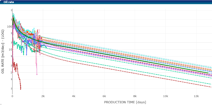
Using the Apply button, the curves are generated for 3 percentiles:

Type Well – Curves generated for type wells P10, P50 and P90 (solid curves in green)

Type Well User defined

The Type Well User defined feature allows the user to configure a type well from variables entered by the user according to the chosen decline model.

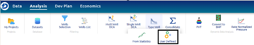Type Well User defined in the main toolbar

Type Well User defined parameters

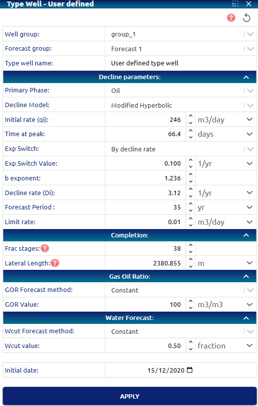Type Well User defined parameters

• Well group: dropdown for selecting the group of wells to choose the forecast

• Forecast group: dropdown for selecting the forecast for use in determining statistics

• Type well name: Name entered by the user for the well type

• Decline parameters:

o Primary phase: dropdown for selecting multi well forecasts primary phase. Options:

    • Oil

    • Gas

o Decline model: dropdown for selecting multi well forecasts decline model. Options:

    • Exponential (Exp)

    • Hyperbolic (H)

    • Modified hyperbolic (MH)

    • Power law exponential (PLE)

    • Stretched exponential (SE)

o Initial rate: initial rate for the type well.

    o Time at peak: time at peak rate, expressed in days.

    o (only for MH decline models) Exp Switch: indicates the condition
      for switching from Hyperbolic to Exponential function. Options: by time
      (time), by decline rate (1/time)

    o (only for MH decline models) Exp Switch value: value to enter according to
      the chosen switch option

    o (only for H / MH / Exp decline models) Di: initial decline
      rate, expressed in 1/yr.

    o (only for H / MH decline models) b exponent: parameter that characterizes
      the form of declination of hyperbolic curves.

    o (only for PLE / SE decline models) n exponent: power-law exponent, describes
      how the rate of decline changes over time.

    o (only for PLE / SE decline models) transition time: tau factor, expressed
      in days. Factor that is related to the characteristic time of decline and
      modulates how the production rate declines over time.

    o Forecast period: Indicates the number of years up to which to forecast.

    o Limit rate: Indicates the minimum rate up to which to forecast.

• Completion:

    o Frac. stages: hydraulic fracturing stages.

    o Lateral Length: effective horizontal length of the well drilled within
      the productive formation.

• Custom Scaling:

 Formulas used for scaling:
    o EUR factor = ((L1-L0)/L0) * Ex +1
    o Qi factor = ((L1-L0)/L0)/2 * Ex +1

    With "L1" being the normalized lateral length input by the user, "L0" the current lateral length and "Ex" the exptrapolation error.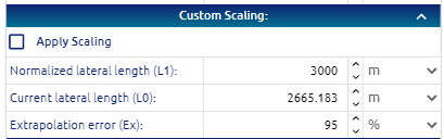

• Gas Oil Ratio:

• GOR forecast method: dropdown for selecting GOR forecasting method. Options:

    o Manual: the following parameters must be entered that will determine
      the GOR curve during the production of the well:

• a parameter: set GOR curvature until GOR max, values between 1 and 20.

• GOR initial value, GOR Max, and GOR Final: characteristic values of the GOR (y axis) to adjust its curve.

• Np@BubblePoint, Np@GOR Max, Np@GOR Final: characteristic production values to adjust the production (x axis) to the GOR curve.

    o Constant: an individual value must be entered for the GOR.

• Water Forecast:

    o Water Forecast method: dropdown for selecting GOR forecasting method. Options:

     o Manual

     o Constant

     o Automatic

• Constant: uses a constant water cut value that must be entered by the user.

• Initial date: production start date for the type well.

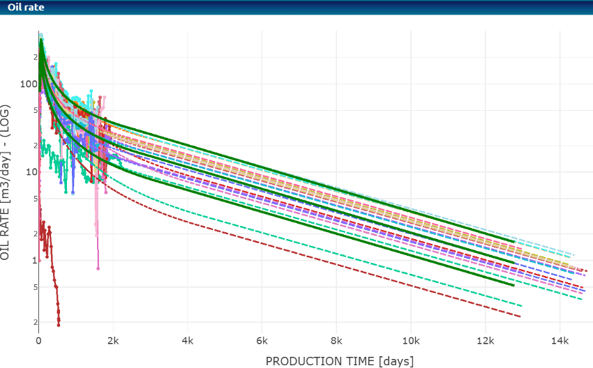
Using the Apply button, the curve is generated for the type well:

Type Well User defined– Curve generated for the type well (solid curve in green)

Detailed Calculations

Swanson’s Mean

Given percentiles P90, P50, and P10, Swanson’s mean is calculated as follows:

Swanson’s Mean = 0.3 x P10 + 0.4 x P50 + 0.3 x P90

P̂

P10/P90

P10/P90

M3 Compliant

Distribution, Percentiles, and Equation Glossary The following procedures and calculations use the vocabulary below:

qi: initial (peak) production rate for the primary phase, from which decline begins.

EUR (Estimated Ultimate Recovery): forecasted final oil or gas recovery volume.

Sample: individual data point corresponding to a qi or EUR value from a single well.

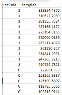
Step 1) Data Sampling Using the Chart Toolbar, the user adds or removes points (wells) from the dataset for analysis.

This creates two lists: included samples and excluded samples. The included samples are then sorted in descending order.

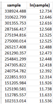
Step 2) Logarithmic Transformation The natural logarithm is computed for each sample value.

Step 3) Percentile Calculation and EDF Construction The corresponding percentile is computed for each sample, allowing construction of the Empirical Distribution Function (EDF).

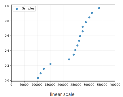
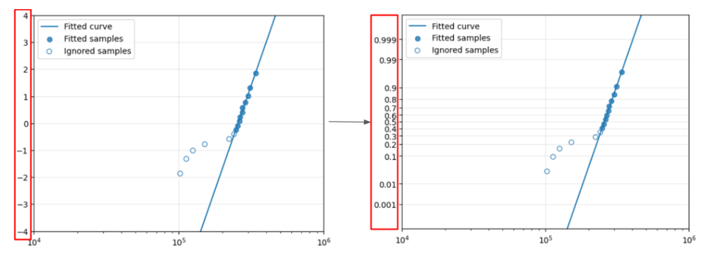
Linear scale

Log scale

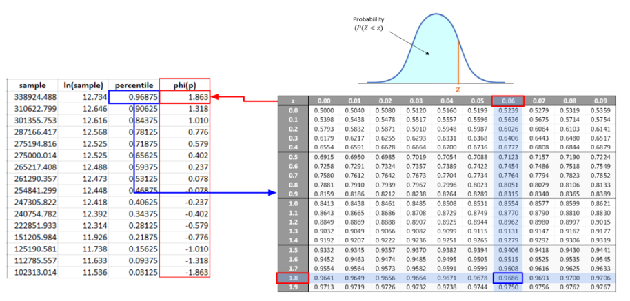
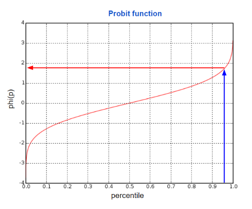
Step 4) Inverse Standard Normal Transformation The inverse value (z-score) of the standard normal distribution is computed for each percentile.

This comes from the probit function curve.

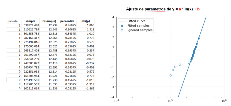
Step 5) Logarithmic Curve Fit A logarithmic curve is fitted to the included samples (x, φ(x)).

Step 6) Y-Axis Transformation to Probit Scale The Y-axis ticks are transformed using the probit function, in the same way as the samples.