Multi well DCA Menu

The Multi well decline curve analysis feature allows the user to forecast a set of wells in an automated way, after setting up the forecast parameters. The feature will be located over ‘Analysis’ tab in the navbar, inside ‘Decline Curve Analysis’ section.

Decline Curve Analysis in the main toolbar

In order to calculate forecasts, it is required that the user has selected some wells for analysis. This means it is necessary for the Multi well DCA feature to have a Wells selection that retrieves the historical data for the selected wells, and a Wells list for displaying/hiding wells.

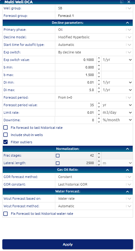
Multi well DCA menu

This menu allows the user to set the parameters for the automated forecast:

• Forecast group: text input for setting a name for a group of multi well forecasts

• Well group: dropdown for selecting the group of wells to forecast Decline parameters

• Primary phase: dropdown for selecting multi well forecasts primary phase. Options:

        o Oil

        o Gas

• Decline model: dropdown for selecting multi well forecasts decline model. Options:

        o Exponential (Exp)

        o Hyperbolic (H)

        o Modified hyperbolic (MH)

        o Power law exponential (PLE)

        o Stretched exponential (SE)

• (only for H / MH decline models) b min / b max: b factor lower and upper boundaries for fitting.

• (only for H / MH / Exp decline models) Di min / Di max: initial decline rate lower and upper boundaries for fitting.

• (only for MH decline model) Exponential switch: dropdown for selecting switch method from hyperbolic to exponential. Options:

        o By time (days)

        o By decline rate (1/yr)

• (only for MH decline model) Exp switch value: input number for setting exponential switch decline rate or time.

• (only for PLE / SE decline models) n min / n max: n exponent lower and upper boundaries for fitting.

• (only for PLE decline model) Decline rate at t=inf: decline rate at infinite time.

• Start time: Available options: Automatic (looks for peak rate and starts forecast), time from peak rate, time before last historical production.

• Forecast period: input number for selecting years to forecast.

• Limit rate: input number for selecting minimum limit rate for the forecast.

• Fix forecasts to last historical rate: checkbox for applying vertical shifting to rates curves to make them pass over last historical rate.

Normalization

• Frac stages: checkbox and input number for applying forecasts rates normalization by frac stages.

• Lateral length: checkbox and input number for applying forecasts rates normalization by lateral length.

Gas oil ratio

• GOR forecast method: dropdown for selecting GOR forecasting method. Options:

     o Manual

     o Constant

     o Automatic

• GOR input values: input numbers for setting ‘Manual’ / ‘Constant’ GOR forecasting

Water cut

• Wcut forecast method: dropdown for selecting Wcut forecasting method. Options:

     o Manual (disabled for now)

     o Constant

     o Automatic

• Wcut input values: input numbers for setting ‘Manual’ / ‘Constant’ Wcut forecasting

• Fix forecast to last historical wcut: …

Once the user has configured the Multi well DCA parameters from the menu and clicked ‘Apply’, the calculated forecast will impact on:

• Map

• Time series plots

• Time series display table

• Well data display table

• Statistics

• Results table

Technical specifications

Forecasts calculation

Primary phase

The chosen primary phase determines whether oil or gas rates will be utilized for forecasting via curve fitting.

Oil as primary phase

Time series used for curve fitting will be:

• x-series: production time

• y-series: oil rate

Gas as primary phase

Time series used for curve fitting will be:

• x-series: production time

• y-series: gas rate

Decline model

The chosen decline model determines which equation will be utilized for forecasting via curve fitting.

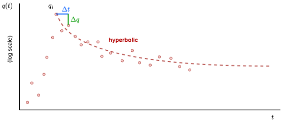
Hyperbolic

The funcion used for curve fitting is based on Arps Hyperbolic decline equation, described in DCA models theory | Hyperbolic

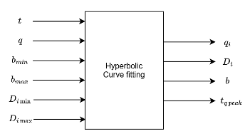Hyperbolic curve fitting parameters

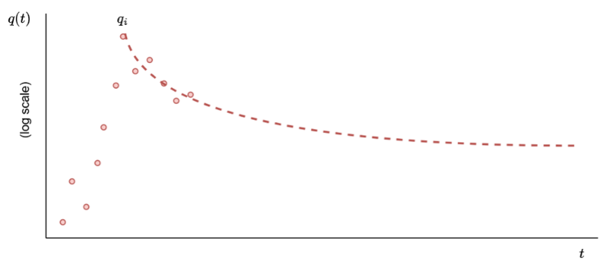Hyperbolic curve fitting

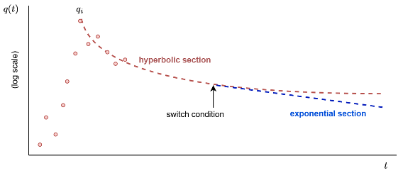
Modified hyperbolic

The funcion used for curve fitting is based on Arps Hyperbolic and Exponential decline equations, described in DCA models theory | Modified hyperbolic

The first section of the Modified hyperbolic is Hyperbolic, but when a certain condition is reached (depending on user’s selection) it must switch to Exponential.

Exponential switch

dropdown is only enabled for Modified hyperbolic decline model, and indicates the condition for switching from Hyperbolic to Exponential function.

Displays the following options:

   • By time [time]

   • By decline rate [1/time]

This dropdown also requires an input number for the user to set the value for the switching condition.

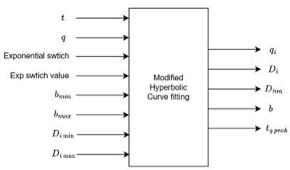Modified Hyperbolic curve fitting parameters

Modified Hyperbolic curve fitting

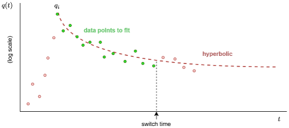
Exponential switch by time

The switch from Hyperbolic to Exponential function must occur at the number of days specified by the user. The forecasting algorithm must first fit the points between the peak rate (qi) and the switch time with a Hyperbolic equation.

Modified Hyperbolic switch by time

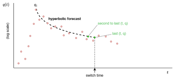
Next, the Hyperbolic function will forecast (based on the parameters provided by the curve fitting process) until the switch time. Then, It is necessary to calculate the decline rate parameter for the exponential section.

This value is calculated from last and second to last hyperbolic forecast data points as:

di_exp = -(last_hyp_rate - second_to_last_hyp_rate) / (last_hyp_rate * (last_hyp_t - second_to_last_hyp_rate))

Modified Hyperbolic switch by time points to use

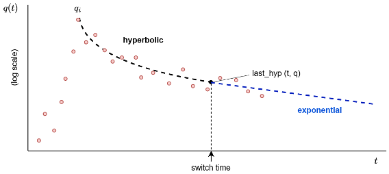
Using the di_exp parameter, the Exponential section is calculated by the equation described in DCA models theory | Exponential assuming

qi = last_hyp_rate

di = di_exp

Modified Hyperbolic, exponential section

Exponential switch by decline rate

The switch from Hyperbolic to Exponential function must occur when the decline curve reaches the decline parameter (D) specified by the user.

First, must decline the rates with a fitted Hyperbolic decline model, to calculate the switch time where the specified decline rate occurs.

Then, the following q_forecast and t_forecast arrays are taken from the hyperbolic forecast, for each historical point, is calculating:

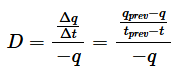
Finally, compare the array of calculated decline rates with the decline parameter (D) specified by the user, and find its position inside the forecasted times array with the Hyperbolic model. Once we have the position of the desired D inside the forecast times array, we could use the Modified hyperbolic with switch by time method.

Modified Hyperbolic, switch by decline rate

Power law exponential

The funcion used for curve fitting is based on Arps Hyperbolic and Exponential decline equations, described in DCA models theory | Power law exponential

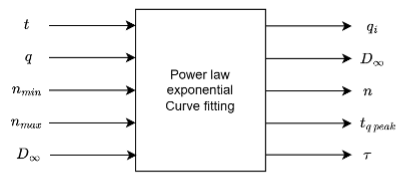Power Law Exponential curve fitting parameters

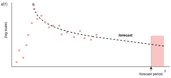
Forecast period

Indicates the number of years up to which to forecast. The forecasted data after the forecast period will be trimmed off. Period time dropdown to set forecast time. From t=0, from last historical data, until fixed date and from peak rate.

Power Law Exponential curve fitting

Limit rate

Indicates the minimum rate up to which to forecast. The forecasted data below the limit rate must be trimmed off.

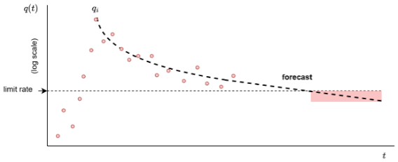Power Law Exponential limit rate

Downtime

Input downtime in % or days per month for the forecast.

Fix forecast to last historical rate

Indicates whether to apply vertical shifting over forecasts to meet the last rate or not. If this parameter is set to ‘true’, the calculation for the shifted rates is:

q_forecast (array) = q_forecast (array) * last_historical_rate / forecasted_rate_at_last_historical_time

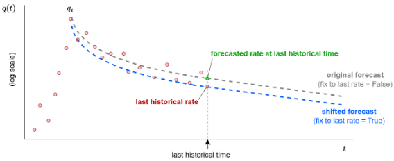Power Law Exponential, last historical rate

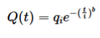
Stretched Exponential

This model is useful in unconventional reservoirs, such as shale, where the decline does not follow a constant rate and presents a more gradual and prolonged decline compared to other decline models such as exponential, hyperbolic or harmonic, described in DCA models theory | Stretched Exponential

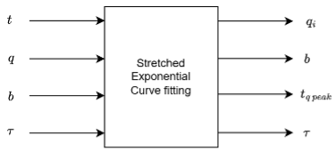Stretched Exponential curve fitting parameters

Model:

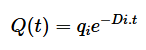
Exponential

The funcion used for curve fitting is based on Arps Exponential decline equation, described in DCA models theory | Exponential

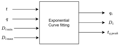
Model:

Gas oil ratio

Calculation options for GOR:

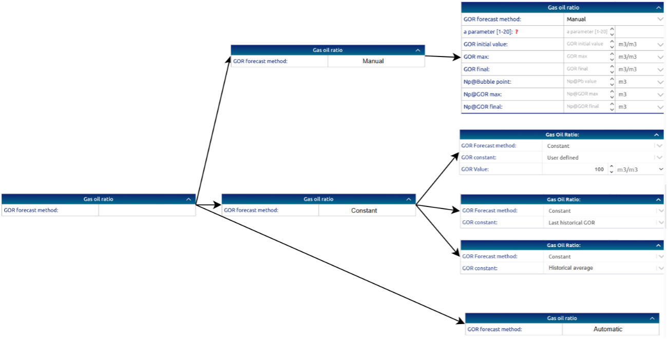Decision tree for GOR calculation