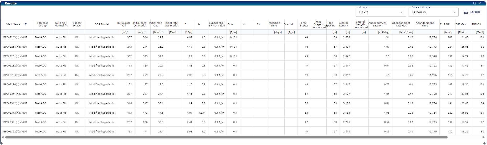
Results
This feature opens a table visualization with the summary of each parameter and results from the calculations done in the DCA module. It contains all the forecast results, curve fitting, models utilized, etc. This table can be exported to an excel file.
-
Well Name – Identifier of the well. Typically follows company naming conventions.
-
Forecast Group – Grouping of wells (by pad, area, or formation) for forecasting or benchmarking purposes.
-
Auto fit / Manual fit – Indicates whether the decline-curve parameters were calculated automatically by the software or entered/adjusted manually.
-
Primary Phase – Main production phase being modeled (Oil or Gas).
-
DCA Model – Type of decline-curve model applied (e.g., Arps hyperbolic, exponential, modified Arps).
-
Initial rate Oil – Starting oil production rate used for the decline model.
-
Initial rate Oil Model – The modeled (fitted) oil rate at time zero from the DCA model.
-
Initial rate Gas – Starting gas production rate used for the decline model.
-
Initial rate Gas Model – The modeled (fitted) gas rate at time zero from the DCA model.
-
Di – Initial decline rate (per time unit) of the production curve.
-
b – Arps’ hyperbolic exponent that controls the curvature of the decline.
-
Exponential Switch Value – Point at which the model switches from hyperbolic to exponential decline (or another form).
-
Dlim – Minimum decline rate used to limit or cap the decline curve (flattening).
-
n – Decline exponent or parameter in modified decline models (if applicable).
-
R² – Statistical coefficient of determination showing the quality of the fit between model and historical data.
-
Transition Time – Time at which the production model transitions between decline segments (for segmented models).
-
D at inf – Asymptotic (infinite time) decline rate — the long-term limit of the decline.
-
Frac Stages – Number of hydraulic fracture stages performed on the well.
-
Frac Stages Normalized – Frac stages normalized to a standard lateral length for comparison between wells.
-
Frac Spacing – Distance between fracture stages along the lateral length of the well.
-
Lateral Length – Length of the horizontal section of the wellbore.
-
Lateral Length Normalized – Lateral length normalized to a common reference for comparisons.
-
Abandonment Rate Oil – Oil production rate at which the well is considered uneconomic and assumed abandoned in the forecast.
-
Abandonment Rate Gas – Gas production rate at which the well is considered uneconomic and assumed abandoned in the forecast.
-
Abandonment Time – Time at which the well reaches its abandonment rate.
-
EUR Oil – Estimated Ultimate Recovery of oil — total oil expected to be produced over the well’s life.
-
EUR Gas – Estimated Ultimate Recovery of gas — total gas expected to be produced over the well’s life.
-
TRR Oil – Technically Recoverable Resource of oil — total oil considered technically recoverable given current technology.
-
TRR Gas – Technically Recoverable Resource of gas — total gas considered technically recoverable given current technology.
-
Creation Time – Date/time stamp when the record, forecast, or model was created in the system.
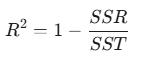
R-squared (R²) Is a statistical measure that represents the proportion of the variance in the dependent variable (in this case, the flow rate) that can be predicted from the independent variable (in this case, time). In simple terms, it tells you how well your model fits the data.
• If R² is 1 (or 100%), the model perfectly predicts the variation and fits the data without errors. This is a “perfect” fit. • If R² is 0, the model predicts none of the data’s variation. This means the model performs no better than a simple average of the data.
How R-squared is calculated:
The calculation of R² typically follows these steps within the fit_model function:
- Model Fitting: The parameters of the decline model (hyperbolic, exponential, etc.) are adjusted to best fit the provided data.
- Prediction Generation: Using the fitted curve and the time values, the function predicts the flow rate for each data point.
- Calculation of Residuals: The difference between the actual flow rate values and the predicted values is calculated. This is known as the Sum of Squares of Residuals (SSR).
- Calculation of Total Variance: The sum of the squared differences between the actual flow rate values and their mean is calculated. This is known as the Total Sum of Squares (SST).
Finally, R² is calculated using the formula: